Variational Reconstruction

Variational reconstruction (TV + NUFFT)¶

This notebook demonstrates vendor-agnostic reconstruction utilities in mrax.reco.

The variational objective solved is:

\[\min_x \; \tfrac{1}{2}\| M\,F\,(S\,x) - y\|_2^2 + \lambda\,\mathrm{TV}(x)\]

• S: coil sensitivity maps (optional)
• F: centered FFT (Cartesian) or NUFFT (non-Cartesian)
• M: sampling mask (Cartesian)

Solves use the project's Optax/proximal tooling (e.g., FISTA + a TV proximal operator).

Dimension note: MRax keeps non-spatial axes explicit (e.g., t, te, ti, offset, b1) and reserves x/y/z for spatial. When data arrives with a single frame axis, importers reshape it to these dimensions and observables are expanded across them during fitting.

import numpy as np
import jax.numpy as jnp
import matplotlib.pyplot as plt

from pathlib import Path
from mrax.reco import build_operator, fftnc, reconstruct_ifft, reconstruct_regrid, reconstruct_variational

mse = lambda a, b: float(np.mean((np.abs(np.asarray(a) - np.asarray(b))) ** 2))

Cartesian: zero-filled vs TV-regularized¶

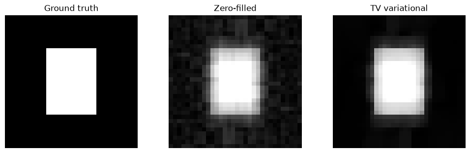
Create an undersampled Cartesian acquisition (keep a small ACS region + every 8th ky line), then compare a zero-filled reconstruction against a TV-regularized variational solve.

Note: regularizer_weight is scale-dependent; for orthonormal FFT k-space this demo uses a small value (around 1e-4).

n = 32
phantom = jnp.zeros((n, n), dtype=jnp.float32).at[8:24, 10:22].set(1.0)
k_full = fftnc(phantom)

# Pseudo-random undersampling mask with fully sampled center
mask = np.zeros((n, n), dtype=bool)
mask[2*n//5:3*n//5, 2*n//5:3*n//5] = True  # fully sampled center
num_samples = n * n // 3  # target number of samples
rng = np.random.default_rng(0)
while mask.sum() < num_samples:
    x = rng.integers(0, n)
    y = rng.integers(0, n)
    mask[x, y] = True

k_us = np.asarray(k_full) * mask

zf = np.asarray(reconstruct_ifft(k_us, mask=mask))
tv = np.asarray(
    reconstruct_variational(
        k_us,
        mask=mask,
        optimizer_name="fista",
        step_size=1.0,
        num_steps=120,
        regularizer="tv",
        regularizer_weight=1e-4,
        tv_iterations=60,
    )
)

print(f"Sampling fraction: {mask.mean():.3f}")
print(f"MSE zero-filled: {mse(phantom, zf):.4g}")
print(f"MSE TV recon:    {mse(phantom, tv):.4g}")

fig, axs = plt.subplots(1, 3, figsize=(10, 3), constrained_layout=True)
axs[0].imshow(np.asarray(phantom), cmap="gray", vmin=0, vmax=1)
axs[0].set_title("Ground truth")
axs[1].imshow(np.abs(zf), cmap="gray", vmin=0, vmax=1)
axs[1].set_title("Zero-filled")
axs[2].imshow(np.abs(tv), cmap="gray", vmin=0, vmax=1)
axs[2].set_title("TV variational")
for ax in axs:
    ax.axis("off")
plt.show()

Sampling fraction: 0.333
MSE zero-filled: 0.01914
MSE TV recon:    0.00813

Cartesian multi-coil SENSE-style example¶

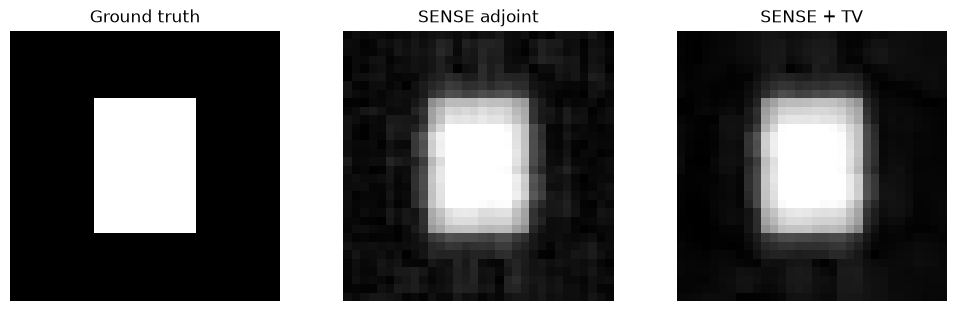
Simulate two smooth coil sensitivity maps and reconstruct the combined image using the explicit coil patterns in the forward model.

Tip: normalizing sensitivities so that sum(|S|^2)=1 improves conditioning in this toy setup.

yy, xx = np.meshgrid(np.linspace(-1, 1, n), np.linspace(-1, 1, n), indexing="ij")
sens1 = np.exp(-2.0 * (xx**2 + yy**2))
sens2 = np.exp(-2.0 * ((xx - 0.4) ** 2 + yy**2)) * np.exp(1j * (np.pi * xx))
sens = np.stack([sens1, sens2], axis=0).astype(np.complex64)

# SOS-normalize: sum(|S|^2)=1.
sens = sens / np.sqrt(np.sum(np.abs(sens) ** 2, axis=0, keepdims=True) + 1e-8)

coil_imgs = np.asarray(phantom)[None, :, :] * sens
k_coils = np.asarray(fftnc(jnp.asarray(coil_imgs)))
k_coils_us = k_coils * mask  # broadcast mask over coils

zf_sense = np.asarray(reconstruct_ifft(k_coils_us, sensitivities=sens, mask=mask))
recon_sense = np.asarray(
    reconstruct_variational(
        k_coils_us,
        sensitivities=sens,
        mask=mask,
        optimizer_name="fista",
        step_size=0.01,
        num_steps=500,
        regularizer="tv",
        regularizer_weight=1e-4,
        tv_iterations=30,
    )
)

print(f"MSE SENSE adjoint: {mse(phantom, zf_sense):.4g}")
print(f"MSE SENSE + TV:    {mse(phantom, recon_sense):.4g}")

fig, axs = plt.subplots(1, 3, figsize=(10, 3), constrained_layout=True)
axs[0].imshow(np.asarray(phantom), cmap="gray", vmin=0, vmax=1)
axs[0].set_title("Ground truth")
axs[1].imshow(np.abs(zf_sense), cmap="gray", vmin=0, vmax=1)
axs[1].set_title("SENSE adjoint")
axs[2].imshow(np.abs(recon_sense), cmap="gray", vmin=0, vmax=1)
axs[2].set_title("SENSE + TV")
for ax in axs:
    ax.axis("off")
plt.show()

MSE SENSE adjoint: 0.01652
MSE SENSE + TV:    0.01418

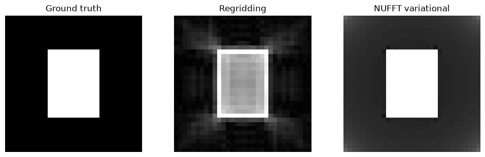
Non-Cartesian example (NUFFT + regridding)¶

When you supply a non-Cartesian trajectory (in cycles/pixel), the operator uses FINUFFT (jax-finufft) for forward/adjoint operations.

• reconstruct_regrid: nearest-neighbor regridding + IFFT preview
• reconstruct_variational: iterative solve with the NUFFT forward model

Trajectory convention: trajectory[:, 0] = kx, trajectory[:, 1] = ky.

num_spokes = 64
num_samples = n

r = np.linspace(-0.5, 0.5, num_samples, endpoint=False, dtype=np.float32)
angles = np.linspace(0, np.pi, num_spokes, endpoint=False, dtype=np.float32)
kx = (r[None, :] * np.cos(angles)[:, None]).reshape(-1)
ky = (r[None, :] * np.sin(angles)[:, None]).reshape(-1)
traj = np.stack([kx, ky], axis=1).astype(np.float32)

# Density compensation is applied by default for non-Cartesian trajectories (simple |k| DCF
# normalized so weights sum to the number of spatial pixels). Pass
# density=np.ones(traj.shape[0]) to disable or provide custom weights.
density = None

op = build_operator(spatial_shape=(n, n), trajectory=traj, density=density)
samples = np.asarray(op.forward(phantom))[0]
scale = np.max(np.abs(samples)) + 1e-8
samples = samples / scale

regrid_img = np.asarray(reconstruct_regrid(samples, traj, spatial_shape=(n, n), density=density))

schedule = [(1e-3, 120)]
tv_lambda = 5e-3
x0 = None
for step_size, steps in schedule:
    x0, stage_history = reconstruct_variational(
        samples,
        spatial_shape=(n, n),
        trajectory=traj,
        density=density,
        optimizer_name="split_bregman",
        step_size=step_size,
        num_steps=steps,
        regularizer="tv",
        regularizer_weight=tv_lambda / step_size,
        initial_image=x0,
        return_history=True,
    )
    if not np.isfinite(np.asarray(stage_history)).all():
        raise RuntimeError("Non-finite loss; lower step_size or clip gradients more.")
    if not np.isfinite(np.asarray(x0)).all():
        raise RuntimeError("Non-finite image; lower step_size or clip gradients more.")
iter_img = np.asarray(x0)

regrid_img = regrid_img * scale
iter_img = iter_img * scale

print(f"MSE regridding: {mse(phantom, regrid_img):.4g}")
print(f"MSE NUFFT iter: {mse(phantom, iter_img):.4g}")

fig, axs = plt.subplots(1, 3, figsize=(10, 3), constrained_layout=True)
axs[0].imshow(np.asarray(phantom), cmap="gray", vmin=0, vmax=1)
axs[0].set_title("Ground truth")
axs[1].imshow(np.abs(regrid_img), cmap="gray", vmin=0, vmax=1)
axs[1].set_title("Regridding")
axs[2].imshow(np.abs(iter_img), cmap="gray", vmin=0, vmax=1)
axs[2].set_title("NUFFT variational")
for ax in axs:
    ax.axis("off")
plt.show()

MSE regridding: 0.07012
MSE NUFFT iter: 0.02874